
ISSN (0970-2083)
ISSN (0970-2083)
Essombo Bathelemy1, Deli Goron1,4 , Cyrille Talla Fotsing1,3, Jean Calvin Seutche1,2*, Achille Clovice Goune1, Jean Luc Nsouandele4, Germain Hubert Ben-Bolie5
1Electrical and Electronic System Laboratory, University of Yaoundé I-Cameroon, Yaoundé, Cameroon
2Department of Physics, University of Maroua, Maroua, Cameroon
3Department of Physics, University of Yaoundé I-Cameroon, Yaoundé, Cameroon
4National Advanced School of Engineering Maroua, University of Maroua–Cameroon, Maroua, Cameroon
5Laboratory of Atomic, University of Yaounde, Yaounde, Cameroon
Received: 26-Oct-2022, Manuscript No. ICP-22-78206; Editor assigned: 01-Nov-2022, PreQC No. ICP-22-78206 (PQ); Reviewed: 15-Nov-2022, QC No. ICP-22-78206; Revised: 23-Nov-2022, Manuscript No. ICP-22-78206 (A); Published: 30-Nov-2022, DOI: 10.4172/0970-2083.006
Visit for more related articles at Journal of Industrial Pollution Control
The major difficulty today is to know exactly how much Greenhouse Gases (GHG) are generated by thermal power plants by using a suitable method and model. These GHG include Carbon Dioxide (CO2), which is an effective contributor to environmental destruction. The method used here is the empirical estimation method of GHG in line with the iso norms of the Cameroonian industrial framework for the determination of the exact emissions in kg of GHG (CO2, CH4 and N2O) from the Oyom-Abang I Thermal Power Plant (TPO) during the years 2016; 2017 and 2018. This method was found to be likely, a daily average of 33.79 kg, 98.13 kg and 26.38 kg for Carbon Dioxide (CO2), Methane (CH4) and Nitrous Oxide (N2O) respectively. The first five days of December were chosen for an error’s estimation study in the GHG inverse modelisation with regard to the amount of electricity produced, we can note that in 2016, 2017 and 2018 we have 11043.6 kWh; 8193.891 and 15268.369 kWh respectively. From these results, we can see that in 2016 and 2017 we have a decrease in production compared to 2018. Given these quantities, the errors in the inverse modelisation of these GHG are: (15,70%; 16,18%) for Carbon Dioxide (CO2 ); (16,18%; 16,99%) for Methane (CH4) and 16,18% for Nitrogen Peroxide (N2O).
Atmosphere, Environment, Gaussian model, Greenhouse Gases, Inverse medialization
Cameroon is a Central African country with significant energy potentials, 13% of which is provided by thermal power plants (Eneo, 2018). It is a signatory to several international environmental conventions edited by Seutche et al. (2015), aimed at limiting air pollution. The production of this energy from thermal power plants has a serious impact on the environment and on our health; through a huge release of greenhouse gases such as carbon dioxide (CO2); for methane (CH4) and for nitrous oxide (N2O) into the atmosphere, which are punctual and sometimes accidental. The production of electricity by burning fossil fuels (HFO and LFO) in thermal power plants in Cameroon is one of the main sources of pollution (Seutche et al., 2019).
This article deals first with the quantification of greenhouse gas’ emissions from the Oyom-Abang I thermal power plant, then with the simulation of greenhouse gas concentrations and finally with the estimation of modelling errors in order to reconstruct the pollution source.These punctual and accidental releases of these greenhouse gases go from catastrophic events and continue to multiply in occurrence: the accident of Chernobyl in Ukraine in 1986, the nuclear power plant of Fukushima Daiichi in Japan in 2011, of the thermal power plant of Oyom-Abang I in 2015 and as well as the explosion of the Lake Nyoss in Cameroon in 1986; haven caused enormous material damages and human loss of lives, in most cases the massive emissions of gases, pollutants and radionuclides from their various sources in the atmosphere. It would therefore be important to know for the species of CO2, CH4 orN2O . How much gas would be emitted into the atmosphere for this purpose; over a given period for the best reconstruction of the pollution source.The reconstruction of the atmospheric tracer source term depends on the equilibrium of the charged information in the observation set and the number of source parameters to be retrieved. As well as the nature of the source-receptor relationship, in order to provide a digital model of Atmospheric Transport (ATM). The source-receiver relationship (Wiiniarek et al., 2012) is:
μ = Hσ +ε ..........(1)
Where is the measurement vector, is the source vector, is the Jacobian matrix of the transport model which is linear in this context for particular gaseous particles; it is clear that H also incorporates the observational context. The vector is called observational error in this paper, it also represents instrumental errors, as well as represented errors. The Jacobian matrix is ill-conditioned, which allows us to state that the relationship is an ill-posed inverse problem according to (Enting, 2002; Wiiniarek et al., 2012). The reconstruction of the source terms of CO2, CH4 and N2O in the Oyam-Abang I thermal power plant critically depends on the results of theoretical and simulated concentrations in the same domain.
In recent years, a number of researchers have paid increasing attention to these problems, both from a theoretical and application perspective, leading to the development of various deterministic techniques proposed and implemented by (Penenko et al., 2002; Lennart and Joakim, 2000 ; Patrick and Piotr, 2006 ; Sapna et al., 2009) and probabilistic ones proposed and implemented by (Jonathan et al., 2007). Probabilistic approaches are limited in their applicability, especially in emergency situations, due to their dependence on prior information and the expensive computerized requirements of sampling approaches. In particular, in case of ill-posed inverse problems where a multimodal solution exists, these techniques are not always able to provide the exact solution. In recent years, the computerized cost of these approaches has been considerably reduced by introducing adjoint concepts originally proposed by (Wiiniarek et al., 2012). In order to overcome the inherent problems, a new ‘renormalisation’ approach has been proposed by (Issartel et al., 2007; Sapna et al., 2009) which is essentially a weighted optimisation, free of any initialization or a priori information on the release and computerized efficiency. However, to date, these techniques have only been used to identify point source emissions (Mei-Kao , et al.,2005).
Description of the Study Area
The OYAM ABANG district is located in the Centre region of Cameroon. The surface occupying the thermal power plant is called OYO. It is an industrial site with a surface area of 1.38296 hectares and its geographical coordinates are (Latitude: 03.52 to 51.7 on Longitude: E 011°28’00.6’’) producing electricity from Heavy Fuel Oil (HFO) and Light Fuel Oil (LFO) injected into CATERPILAR3516B WARTSILA VASA 18V32LN engines. The company involved in this production is Eneo (Energy Cameroon) so the source of information is (Eneo, 2018; Seutche et al., 2019).
For this geographical environment (Seutche et al., 2019) indicate, thanks to fixed and itinerant measurements of meteorological parameters, the Oyam Abang basin experiences each day a period of study of two local meteorological phenomena in the absence of marked synoptic wind; which is the rule in this region:
• The phenomenon of thermal breezes.
• The presence of a temperature inversion.
In addition, the flow of cold air along the slopes accentuates the inversion phenomenon and allows the installation of a thin, calm or weakly ventilated lake of cold air. The topographic configuration offers few escape routes for the cold air. It therefore accumulates at the bottom of the basin with the pollutants emitted (Fig. 1).

Figure 1: OYOM-ABANG in the city of Yaoundé-Cameroon.
In this section, we introduce the methodology of error estimation on the inverse modelling of air pollutants. For this purpose, the study conducted in the Oyom-Abang I thermal power plant allowed us to collect the data on the amount of fuel for three years (2016-2018). The target species to be reconstructed are: CO2, CH4 and N2O.
Methodology for Estimating Greenhouse Gas Emissions: CO2, CH4 and N2O
In this section, we introduce the methodology for estimating errors in the inverse modelling of Greenhouse Gases (GHG). For this purpose, the study conducted in the Oyom-Abang I thermal power plant allowed us to collect the data on fuel quantity for three years (2016- 2018). The target species to be reconstructed are: CO2, CH4 and N2O.
Methodology for Processing Greenhouse Gas Estimation Data
The estimation of these emissions is done by means of a database in which all information relating to emissions has been compiled at the basic unit level. It takes into account 7 parameters (Seutche et al., 2015).
• The type of heat engine
• Fuel type
• Geographical area
• Fuel consumption per unit of electricity supplied
• Engine running time
• The percentage of chemical elements in the fuel oil
• And the technology for controlling CO2, CH4 and N2O emissions.
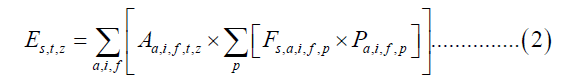
A more detailed description of a substance, an operating time interval and a geographical entity is illustrated by the formula in equation 2 (Fontelle, 2010):
The emissions of a given activity are expressed by the formula in equation 3 (Fontelle, 2010):
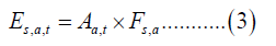
E is the relative emission of the substance and activity at time t and is expressed in CGE.
Aa,t and Fs,a in equation (3) are determined by eight (08) fine combinations of activity typically involving operation, technology and product (Seutche et al., 2019). From this expression, we return to expression (3) by considering particular models such as the activity model where emissions are reported as a single parameter in the activity matter. Large point sources such as thermal power plants are studied individually. In Cameroon, the maximum load hours during emissions in the study area are thus taken into account (Fig. 2). The method used is based on the principle of conservation of matter and can be applied to the emissions of CO2, CH4 and N2O by using the following formula of the second level according to the Cameroonian political context by the relation (4) (Fontelle, 2010;Piotr,et al.,2006; Robertson, et al., 1982):
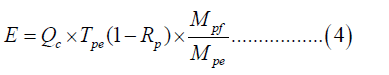

Figure 2: Analytical solution for identifying pollutant sources using the Gaussian method. Note: ( ) 2016; (
 )2017; (
 )2018.
In this expression, E the emission of the polluting substance in the form of the outlet to the atmosphere is expressed in kilograms. The daily, monthly and annual emissions of the Oyom-Abang I thermal power plant were successively calculated on the basis of specific consumption units of each type of fuel oil, factors related to pressure, representatives and their life span, more associated to the regional level. In general, the equation for estimating greenhouse gas emissions is as follows (S. Nazari et al., 2010):
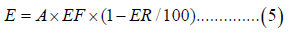
E: Quantity of polluting emissions
A: Activity rate (production quantity of the industrial unit: tonnage of cement produced or electricity produced in terms of kWh)
EF: Emission factor
ER: Emission factor: Total percentage of emission reduction, which is zero if pollution abatement systems are not used.
In thermal power plants, the emission factor is expressed as a function of the intensity of the pollutants produced or the thermal energy consumed or the energy produced in the plant. Table 1 gives a summary of the emission factors used according to the type of fuel used in the Oyoma- Abang I thermal power plant, according to (EPA 2004; Nazari S et al., 2010) in their various research works.
| FUEL type | Emission factor g.kWh-1 | ||
|---|---|---|---|
| CO2 | CH4 | N2O | |
| Heavy oil | 1025±16 | 3000 | 600 |
| Gaz oil | 1083±17 | 3170 | 634 |
Table 1. Average emission factors of CO2, CH4 and N2O in thermal power plants in Cameroon (FONTELLE, 2010).
Operating time, energy production in the Oyom-Abang I thermal power plant (2016 to 2018)
In TPO I, the engines operated at full speed between 18 and 22 hours, during which time consumption and pollution are at their highest (Fig. 2).
Modelling of Atmospheric Dispersion Simulation
The approach taken here to estimate the source of a gas release from measurements requires simulating the transport of greenhouse gases from the various engines in the air sampled by the measuring instrument backwards in time. It is therefore necessary to record the concentration of the gas just at the exit of the Chemins. Note that the chimney is located at a height of 32 metres. The model for simulating the concentration of greenhouse gases in the atmosphere is based on the advection-diffusion process, which is used here to describe the fate of the transport in the framework of integrate inverse modelling developed by (Seinfeld JH, 1986). Equation (6) describes the phenomenon.

Where C(x,y,z) is the stack concentration in (kg), Kx- ,Ky,Kz the diffusion coefficients in the x, y, z direction respectively in (m2/s) and u,v,w the wind speeds in the, is the GHG source.
The analytical solution of this equation is one fundamental importance to the understanding and description of physical phenomena (Pasquill and Smith, 1993) and is generally used to examine the accuracy and performance of numerical solution approved in the work (Runca and Malguzzi, 1981; Bolzern et al., 1982). In this paper, we present an analytical treatment of the advection-diffusion equation under the assumption that the distribution of the greenhouse gas concentration in the crosswind direction has a Gaussian form. Therefore, the discretization method used here is the space-centred time progressive finite difference method (Runca, et al., 1975).
The initial concentration will then take the following value:

For the boundary conditions it is assumed that:
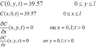
The term Vd encompasses two terms: the dry and wet deposition as the GHG passes through the stack and is given by equation (7) used by (Moreira et al., 2009; Essa et al., 2014; Moreira, et al 2005).
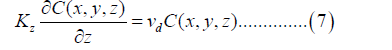
Where Vd is the sum of the dry deposition rate (Vdsec) and the wet deposition rate (Vdhumide) of the GHG in the stack, therefore we have the following:
The Table 2 below gives us for different species of GHG (carbon dioxide CO2, methane CH4 and nitrous oxide N2O) the value of deposition velocities Vd.
| Greenhouse gases | Deposition velocity Vd(m.s-1) |
|---|---|
| Carbon dioxide: CO2 | 0 .5 |
| Methane: CH4 | 0.2 |
| Nitrous oxide:N2O | 0.01 |
Table 2. Average emission factors of CO2, CH4 and N2O in thermal power plants in Cameroon (Fontelle, 2010).
Methodology of Source Reconstruction
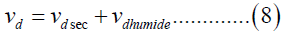
Equation (1) of the source-receiver relationship is an illposed inverse problem (Wiiniarek et al., 2012) and in addition the means of remote sensing being essentially unavailable, as in the case of radionuclides (Bocquet, 2005) the number of observations will therefore be limited. To compensate for the lack of constraints and to better parameterize the source with a limited number of variables, it is necessary to use so-called parametric methods that will regularize the inverse problem and even allow the calculation of the probability density function of the parameters by stochastic sampling techniques used by (Delle Monache et al., 2008; Yee et al., 2008). By applying the variational approach on the source term σk using theoretical concentrations, the modelling of the atmospheric dispersion and deposition of the species to be considered will be considered, a method described in two publications including (Wiiniarek et al., 2012; Saunier et al., 2017; Shou-dong, et al., 2005) assume that the measurement vector μ in d can be described as a linear problem. The observation errors defined in equation (1) are generally assumed to be Gaussian with a normal distribution (Saunier et al., 2017):
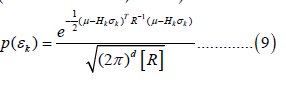
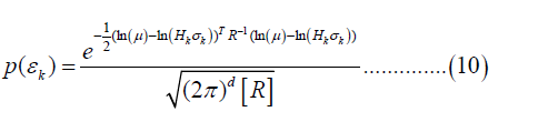
 is the covariance matrix of the R= E (observation errors where (R) is the determinant. A strong disadvantage of Gaussian observation errors is that they give more weight to the higher concentration values than to the lower ones because it is the value of the model-measurement difference that is taken into account in the probability density function (pdf). Several solutions have been proposed to overcome this difficulty (Saunier et al., 2017). The most likely one is to choose a log-normal distribution of observation errors developed by (Rachid and Marc, 2009) with a probability density (pdf) defined by:
Assuming lognormal observation errors, the application of Bayesian inference leads to:
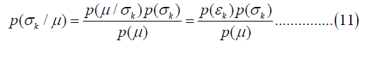
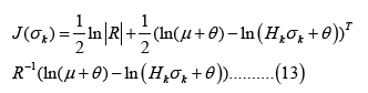
From this inference, to obtain the maximum posteriori estimate p (σk/μ), the likelihood p (μ/σk) must be maximized, which amounts to maximizing p (μ/σk) and minimizing the following cost function J (σk):

Where J (σk) measures the log difference between the model predictions Hk σk and the actual measurement μ as described in (Saunier et al., 2017). The main drawback of log-normal observation errors is that they place too much emphasis on very small concentration values. One way to mitigate the influence of small concentration values is to introduce a threshold in the cost function as follows:
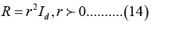
These tempers the values of J (σk) if there are large differences between the observed and simulated concentrations, especially for low concentrations with values just above the detection limit. In this paper we will choose to consider the log-normal observation errors while a simple parameterization for the R matrix is used. It is assumed that R is diagonal and that the error variance is the same for all elements of the diagonal (homoscedasticity property) (Wiiniarek et al., 2011):
Indeed, by minimizing J (σk), this corresponds to minimizing by writing:
The latter expression is based on a number of more sophisticated models for the statistics of observation errors. With a small number of observations, they may be less robust and too artificial.
The main inputs to the model: The Gaussian model supports a number of different modules and configuration options that allow the effects influencing the identification of a source to be taken into account. A number of assumptions can thus be made for each model. In this work, tests have been carried out in order to adjust the modelling parameters to the local context. Some of these are outlined below.
Meteorological Data
The meteorological pre-processor integrated in the Gaussian model calculates the atmospheric boundary layer (AL) parameters from different data sets, for example wind speed and direction, date, time, cloud cover, heat flux density and AL height, etc. The meteorological data used can be raw, on an hourly or daily basis, or derived from statistical analysis. An hourly sequential weather file (for the days of December 2018) was created from data measured by the Ekounou meteorological station (a district in the Central Cameroon region) and controlled by the Ministry of Transport. The parameters reported are: temperature, wind speed, direction and cloud cover. Each month, the daily average temperature as in (MinTransport, 2022) varies between 24°C and 29°C, the cloud cover is 80% on average, the wind speed varies between 2 and 19 km/h in the west according to the wind rose Fig. 3. The wind rose is related to a circle which can be divided into 4, 8, 16 or 32 parts. Like the trigonometric circle, the main directions are: North is 0 or 360°, East is 90°, South is 180° and West 270° (Rachid, et al., 2009; Tirabassi, et al., 2008).

Figure 3: Wind rose around the Oyom-abang thermal power plant (MinTransport, 2022).
The Fig. 3 shows the daily temperatures for the month of December 2018. These temperatures were chosen to observe the influence of temperature on the concentration of GHG in the stack. The highest temperatures are between 10:00 Am and 3:00 pm and the lowest between 4:00 pm and 09:00 am. Fig. 4 shows us the temperature variation during the month of December 2018.

Figure 4: Temperature variability during December 2018.
From the data collected in the company Eneo during my internship from December 15, 2018 to February 15, 2019, the processing of these data using Microsoft Excel 2016 and MATLAB software version 2016a allowed us to formally illustrated the production of energy in Kilowatt- hour (kWh) in the thermal power plant of Oyom- Abang-Yaounde. Fig. 5 shows the electricity production for the years 2016, 2017 and 2018.

Figure 5: Electricity production for the years 2016; 2017 and 2018 in the thermal power plant of Oyom-Abang I- Yaoundé in Cameroon. Note: () 2016; () 2017; () 2018
It should be noted that TPO I is an energy production unit, with 13 MW (Eneo, 2018) of energy production at the time of its implementation. This energy production shows the operation of the different engines of the power plant. The energy is produced in this unit daily in the interval 5:00 P.M. to 10:00 P.M. where we observe a very maximum production.
We see that the most important months in terms of high production for these three years are November, December, January and February. We observed a very important production:
In 2016, the maximum production was observed in the months of December and March, with 1241 kWh and 1481 kWh. This increase was due to the presence of the dry season and the hectic holiday season when people consume considerable amounts of electricity in their households (Seutche et al., 2015). The least unfavourable months are from April to October, where we observed an exponential decrease in electricity production. This is due to the increased water flow in the rivers, which implied a positive impact on electricity production in the hydroelectric dams in Cameroon and in this case the SONGLOULOU dam (located on the Sanaga-Cameroon River and having a production capacity of 384 MW, so its reservoir level is 528 m) (Eneo, 2018).
In 2017, the maximum production was observed between the months of November and December, with 2136 and 2654 kWh. This increase was due to the presence of the dry season and the busy holiday season. The production was less maximal between January and March. On the other hand, we observed an exponential decrease from April to September. This decrease is due to the increased water flow in the rivers, which had a positive impact on the production of electricity in the hydroelectric dams in Cameroon.
In 2018, all three engines were already in full operation, so there was considerable production in all months. But the maximum production was observed between October and January, with up to 2514 kWh in December. This increase was due to the presence of the dry season and the hectic period of the end of year festivities where people consumed a considerable amount of electrical energy in their households. The months where we see a decrease in energy use, are from February to August. This is due to the increased water flow in the rivers, which had a positive impact on the production of electricity in the hydroelectric dams in Cameroon.
Fig. 6 shows the cumulative electricity production during the years 2016, 2017 and 2018 in CTO I. In TPO I, the years 2016 and 2017 saw energy production of 11043.6 kWh in 2016 and 8193.891 kWh in 2018, while in 2018 we had a cumulative production of 15268.369 kW/h. We can therefore see that in 2018 the three engines of the thermal power plant were already running due to the very high production. On the other hand, in 2016 and 2017 the power plant had only one engine running since the incident in 2015.

Figure 6: Cumulative electricity production during the years 2016; 2017 and 2018 in the Oyom-Abang I thermal power plant.
Results of Greenhouse Gas Emissions in TPO I
In the years 2016, 2017 and 2018, the GHG emissions assessed in the TPO are considerable. The estimation of GHG emissions was done on the basis of the methodology presented by the IPCC and the results of these emissions took into account the IPCC emission factors. Fig. 7 showing us the amount of emissions in kg of the different greenhouse gases (emission of CO2; emission of CH4 and emission of N2O).

Figure 7: CO2 emissions in the years 2016; 2017 and 2018. Note: () 2016; () 2017; () 2018.
Fig. 7 shows us that CO2 emissions are a function of HFO consumption with 1.025 times electricity production (Benny et al., 2018; Seutche et al., 2015). We find that:
In 2016 the concentration is maximum in March with 1272 kg and minimum in January 527.8 kg.
In 2017 the concentration is maximum in the month of December 2171 kg and 0 kg from the month of May until August.
In 2018 the concentration is highest in December (2674.90 kg) and lowest in July (1186 kg).
This variation in emission is simply due to high fuel consumption (HFO and LFO) resulting in a production up to 1481 kWh in the month of March in 2016; 2654 kWh in December 2017 and 2514 kWh in December 2018 (Figs. 8 and 9).

Figure 8: CH4 emissions in the years 2016; 2017 and 2018. Note: () 2016; ()2017; () 2018

Figure 9: N2O emissions for the years 2016; 2017 and 2018. Note: () 2016; ()2017; () 2018
From the above, the combustion of HFO and LFO in the different engines of the TPO implies a considered release of GHGs. The level of emission of these GHG on the engines varies according to the amount of fuel burnt in the engines and consequently to the operating time of the engines during combustion (Fig. 2). We can therefore note that:
In 2016 the concentration of Methane (CH4) and Nitrogenperoxide (N2O) are maximum in the month of March with 4443.63 kg and 888.72 kg respectively and minimum in the month of January with 1544.64 kg and 308.92 kg respectively.
In 2017 the concentration of Methane (CH4) and Nitrogenperoxide (N2O) are maximum in December, 6354.33 kg and 888.72 kg respectively, and minimum from May to August.
In 2018 the concentration of Methane (CH4) and Nitrogenperoxide (N2O) are maximum in December, with 7543.02 kg and 1508.60 kg respectively are minimum in July, 3469.89 kg and 693.97 kg respectively.
This interpretation triggers a positional analysis assuming that Methane (CH4) and Nitrogenperoxide (N2O) concentrations are highest in December 2018 and lowest in August 2017 (Yee, et al., 2008; Yu,et al.,2008).
Observed and Simulated Emissions in the Oyom- Abang I Thermal Power Plant (TPO I)
The analysis of the different GHG emissions in the Oyom- Abang thermal power plant during the years 2016; 2017 and 2018 were presented using the empirical method of the second level given the industrial rank of our country Cameroon (developing country). The results show that methane (CH4) emissions are considerable. According to the second report of the Intergovernmental Panel on Climate Change (Benny et al., 2021), (CO2). In our current context, for the determination of GHG estimation errors in TPO I, we used two methods: The empirical GHG estimation method of the second level to give in terms of concentration the amount of GHG at the plant for days 1st, 2nd, 3rd, 4th and 5th December 2018 (Fig. 10). The second method consists of using MATLAB software version 2016b to run a simulation by inverse modelling of the theoretical concentrations and to calculate and record the values.

Figure 10: Greenhouse Gaz (GHG) emissions in kg for the first five days of December 2018. Note: (  ) CO2; (
 ) CH4; (
 ) N2O
) N2O
The simulations of GHG dispersion in the Oyom-Abang I thermal power plant were conducted to compare the simulation results with the available measurement data on daily GHG deposition. The simulated emissions for the first 5 days of December 2018 are presented in the following Figs. 11A-11C, 12A-12C, 13A-13C, 14A-14C and 15A-15C:

Figure 11A: Simulations of Greenhouses Gaz transport on 1st December 2018 from TPO I simulation of CO2.

Figure 11B: Simulations of Greenhouses Gaz transport on 1st December 2018 from TPO I simulation of CH4.

Figure 11C: Simulations of Greenhouses Gaz transport on 1stDecember 2018 from TPO I simulation of N2O.

Figure 12A: Simulations of Greenhouses Gaz transport on 2nd December 2018 from TPO I simulation of CO2.

Figure 12B: Simulations of Greenhouses Gaz transport on 2nd December 2018 from TPO I simulation of CH4.

Figure 12C: Simulations of Greenhouses Gaz transport on 2nd December 2018 from TPO I simulation of N2O.

Figure 13A: Simulations of Greenhouses Gaz transport on 3rd December 2018 from TPO I simulation of CO2.

Figure 13B: Simulations of Greenhouses Gaz transport on 3rd December 2018 from TPO I simulation of CH4.

Figure 13C: Simulations of Greenhouses Gaz transport on 3rd December 2018 from TPO I simulation of N2O.

Figure 14A: Simulations of Greenhouses Gaz transport on 4th December 2018 from TPO I simulation of CO2.

Figure 14B: Simulations of Greenhouses Gaz transport on 4th December 2018 from TPO I simulation of CH4.

Figure 14C: Simulations of Greenhouses Gaz transport on 4th December 2018 from TPO I simulation of N2O.

Figure 15A: Simulations of greenhouses gas transport on 5th December 2018 from TPO I simulation of CO2.

Figure 15B: Simulations of greenhouses gas transport on 5th December 2018 from TPO I simulation of CH4.

Figure 15C: S imulations of greenhouses gas transport on 5th December 2018 from TPO I simulation of N2O.
Table 3 below gives us the summary of the quantity in kilograms of the concentration of the different GHGs emitted in the Oyom-Abang I thermal power plant.
| Date | Observed emissions | Simulated emissions | ||||
|---|---|---|---|---|---|---|
| CO2 | CH4 | N2O | CO2 | CH4 | N2O | |
| 1st Dec | 7938625 | 232,35 | 46,47 | 66.54067 | 194.753 | 38.95066 |
| 2nd Dec | 6,70,555 | 196,26 | 39,252 | 56.17031 | 164.5028 | 32.90062 |
| 3rd Dec | 67,59,875 | 197,85 | 39,57 | 56.98638 | 165.8355 | 33.16716 |
| 4th Dec | 10,75,635 | 314,82 | 62,964 | 90.15852 | 263.8784 | 52.77574 |
| 5th Dec | 1,23,984 | 362,88 | 72,576 | 103.922 | 304.1617 | 60.8324 |
Table 3. Summary of observed and simulated theoretical emissions for the first five days of December 2018.
These different values make it possible to say that the releases of these GHG on the TPO are of three types: Carbon dioxide (CO2), Methane (CH4) and nitrous oxide (N2O). A number of questions can be asked about all the thermal power plants in the interconnected network of Cameroon in relation to the quantity of GHGs emitted. Is it measurable? Can we define a scenario over 50 years to control this pollution? If so, what measures should be taken to reduce or partially mitigate this danger to the environment? To this end, we chose to conduct a five- day study to evaluate the squared errors of the various GHGs from the TPO during the month of December 2018 (Tables 3 and 4).
| Date
|
Greenhouse gases
|
||
|---|---|---|---|
| Carbon dioxide (CO2)
|
Methane (CH4)
|
Nitrous oxide (N2O)
|
|
| 1st Dec
|
16,18%
|
16,18%
|
16,18%
|
| 2nd Dec
|
16,23%
|
16,99%
|
16,18%
|
| 3rd Dec
|
15,70%
|
16,18%
|
16,18%
|
| 4th Dec
|
16,18%
|
16,18%
|
16,18%
|
| 5th Dec
|
16,18%
|
16,18%
|
16,18%
|
Table 4. Summary of observed and simulated theoretical emissions for the first five days of December 2018.
Table 4 above shows the squared errors of the different GHG for the first five days of December 2018 between the observed and simulated concentrations. We can see that for carbon dioxide (CO2) the error varies between 15.70% and 16.18%; for methane (CH4) the error varies between 16.18% and 16.99% and for nitrous oxide (N2O) we find an error of 16.18%.
From an analysis and interpretation, we can say that these percentages for the reconstruction of a source destroyed by fire or during a disaster the source can be reconstructed (Wiiniarek et al., 2012).
The analysis by the inverse method confirms that the production of electricity from heavy and light fuel oil by combustion in thermal power stations has an unfavourable environmental balance
The error results of the inverse modelling (at the local scale) of the propagation of Greenhouse Gases (GHG) from the conditional sources of the Oyom-Abang I thermal power plant located in the city of Yaoundé, Centre- Cameroon region, taking into account the accepted values of the simulation parameters, show a good agreement with the measurement data provided by the Eneo company. Based on the GHG estimation method (empirical method), we claim that the indices used to better control the quantification of consumption and emissions are good and allow us to better understand the methods of GHG assessment at the exit of the chimneys of the Oyom- Abang I thermal power plant. As a first solution to reducing the huge amounts of greenhouse gases in the atmosphere, we advocate a more regular and rigorous sustained study of the maintenance system. This is followed by decarbonization and pre-treatment of the fuel before injection into the cylinders and finally the largescale application of methods related to emission control technology.
The simulation in terms of concentration of these different gases gives satisfactory results compared with the literature and the errors on the modelling were approved close to reality considering the comparison with the work of the estimated error of the inverse modelling for Ruthenium-106 2017. For our different greenhouse gases, we found errors of for carbon dioxide (CO2); for methane (CH4) and for nitrous oxide (N2O). These errors in GHG concentrations cause a significant accumulation of energy in the form of heat at the earth’s surface, of which 1% is trapped in the atmosphere. It is this proportion that is the main cause of the global warming observed since 1850. This strategy of control and characterization of emissive sources should already be put in place to better ensure environmental monitoring, as the permanent increase in the content of these gases at the current rate is actively contributing to the increase in morbidity and mortality rates worldwide. Therefore, a more advanced energy transition policy is urgently needed.
This work was supported by the University of Yaoundé I - Cameroon. The work carried out in the framework of this draft paper was also supported by the physics laboratory of the Ecole Normale Supérieure of Yaounde under the supervision of Professor Beguide Bonoma (Head of the physics department of this school); by the energy and thermal engineering laboratory of the Ecole National Polytechnique of Maroua under the supervision of Professor Nsouandele Jean-Luc. The data was taken by the company in charge of electricity in Cameroon (Eneo) and permission was granted by its former director general Joël Nana Kontchou, in one of its production units (Oyom- Abang thermal power plant) supervised by the director of the power plant at the time Guy Thomson. The work of analysis, interpretation, results and writing was done in the Energy, Electrical and Electronic System Laboratory, Research and Training Unit of Physics, University of Yaoundé I- Cameroon, during a period of 6 months.
The authors declare that they have no known competing financial interests or personal relationships that could have appeared to influence the work reported in this paper.
[Crossref][Google Scholar] [PubMed]
[Crossref][Google Scholar] [PubMed]
[Crossref][Google Scholar] [PubMed]
[Crossref][Google Scholar] [PubMed]
Copyright © 2025 Research and Reviews, All Rights Reserved